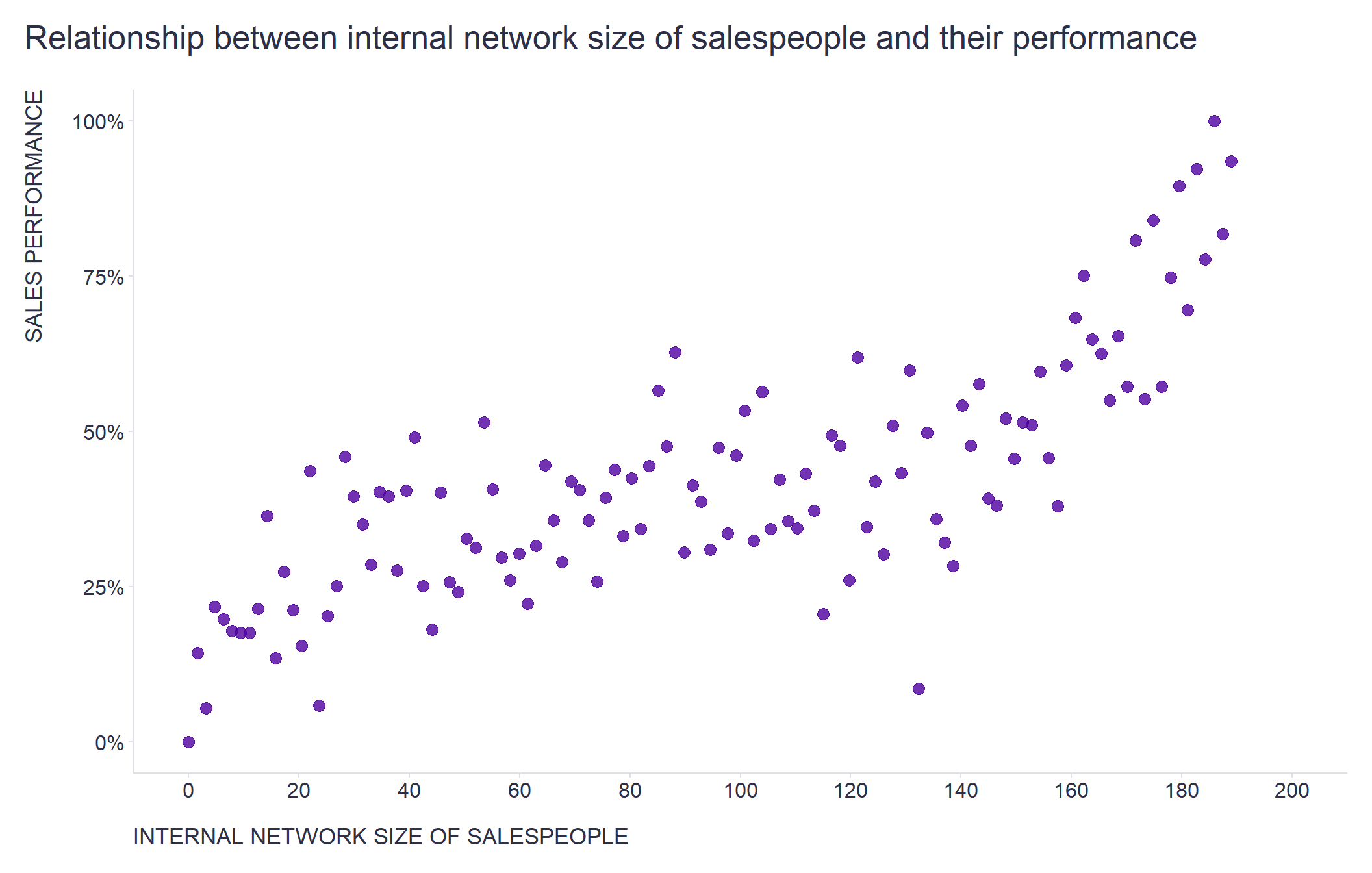
When correlating collaboration metrics with business criteria that our clients are interested in, such as the size of the internal network of salespeople vs. their sales performance, we often encounter the question of where the breakpoint is when people start to score significantly higher/lower on a given criterion.
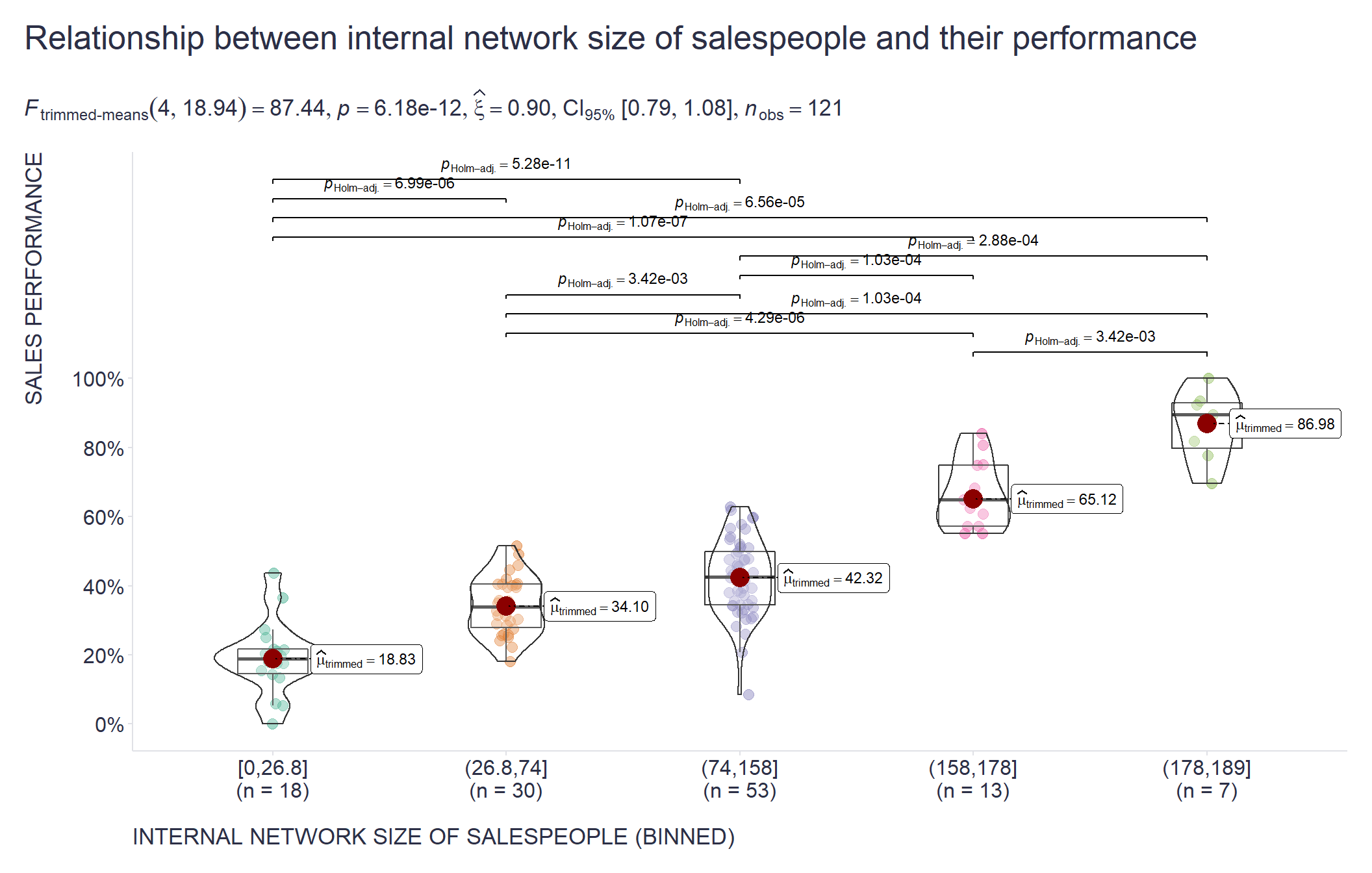
To answer this question, I find very handy the Conditional Inference Tree algorithm - a non-parametric class of decision trees that, unlike traditional decision trees, use a significance/permutation test (corrected for multiple testing) to select covariates to split and recurse the variable.
When applied to just one numerical predictor, it will provide a set of partitions that allow you to split that predictor into bins in such a way that you end up with statistically significant differences between some of the identified bins. With this information in hand, it is much easier for you to find the “sweet spots” (there may be more than one) where the criterion starts to behave differently in relation to the predictor values. See charts below for illustration.
Show code
# uploading libraries for data manipulation and visualuzation
library(tidyverse)

# defining normalize function
normalize <- function(x) {
  return ((x - min(x)) / (max(x) - min(x)))
}


# creating artificial dataset with internal network size and sales performance variables
internalNetworkSize = seq(-6, 6, 0.1)
salesPerf = 1*(internalNetworkSize**3) + 2*(internalNetworkSize**2) + 1*internalNetworkSize + 3
salesPerf_noise = 70 * rnorm(mean = 0, sd = 1, n=length(salesPerf))
salesPerformance = salesPerf + salesPerf_noise

# putting data into dataframe and making some transformations of the variables
data <- data.frame(
  internalNetworkSize = internalNetworkSize,
  salesPerformance = salesPerformance
) %>%
  dplyr::mutate(
    internalNetworkSize = normalize(internalNetworkSize),
    salesPerformance = normalize(salesPerformance),
    internalNetworkSize = internalNetworkSize*189,
    salesPerformance = salesPerformance*100
  )

# visualizing relationship between internal network size and sales performance
ggplot2::ggplot(data = data, aes(x = internalNetworkSize, y = salesPerformance)) +
  ggplot2::geom_point(color = "#4d009d", size = 3, alpha = 0.8) +
  ggplot2::labs(
    x = "INTERNAL NETWORK SIZE OF SALESPEOPLE",
    y = "SALES PERFORMANCE",
    title = "Relationship between internal network size of salespeople and their performance"
  ) +
  ggplot2::scale_y_continuous(labels = scales::number_format(suffix = "%")) +
  ggplot2::scale_x_continuous(breaks = seq(0,200, 20), limits = c(0,200)) +
  ggplot2::theme(plot.title = element_text(color = '#2C2F46', face = "plain", size = 19, margin=margin(0,0,20,0)),
                 plot.subtitle = element_text(color = '#2C2F46', face = "plain", size = 13, margin=margin(0,0,15,0)),
                 plot.caption = element_text(color = '#2C2F46', face = "plain", size = 11, hjust = 0),
                 axis.title.x.bottom = element_text(margin = margin(t = 15, r = 0, b = 0, l = 0), color = '#2C2F46', face = "plain", size = 13, lineheight = 16, hjust = 0),
                 axis.title.y.left = element_text(margin = margin(t = 0, r = 15, b = 0, l = 0), color = '#2C2F46', face = "plain", size = 13, lineheight = 16, hjust = 1),
                 axis.title.y.right = element_text(margin = margin(t = 0, r = 0, b = 0, l = 15), color = '#2C2F46', face = "plain", size = 13, lineheight = 16, hjust = 0),
                 axis.text = element_text(color = '#2C2F46', face = "plain", size = 12, lineheight = 16),
                 axis.line.x = element_line(colour = "#E0E1E6"),
                 axis.line.y = element_line(colour = "#E0E1E6"),
                 legend.position= "bottom",
                 legend.key = element_rect(fill = "white"),
                 legend.key.width = unit(1.6, "line"),
                 legend.margin = margin(0,0,0,0, unit="cm"),
                 legend.text = element_text(color = '#2C2F46', face = "plain", size = 10, lineheight = 16),
                 legend.background = element_rect(fill = "transparent"),
                 panel.background = element_blank(),
                 panel.grid.major.y = element_blank(),
                 panel.grid.major.x = element_blank(),
                 panel.grid.minor = element_blank(),
                 axis.ticks.x = element_line(color = "#E0E1E6"),
                 axis.ticks.y = element_line(color = "#E0E1E6"),
                 plot.margin=unit(c(5,5,5,5),"mm"),
                 plot.title.position = "plot",
                 plot.caption.position =  "plot"
  )
Show code
# uploading libraries for ctree algorithm and visualization of the results of statistical tests
library(partykit)
library(ggstatsplot)

# defining formula
fmla <- as.formula("salesPerformance ~ internalNetworkSize")

# binning internal network size variiablle using ctree algorithm
ctree <- partykit::ctree(
  fmla,
  data = data,
  na.action = na.exclude,
  control = partykit::ctree_control(minbucket = ceiling(round(0.05*nrow(data))))
)

# plotting resulting tree
#plot(ctree)

# number of identified bins
#bins = partykit::width(ctree)

# extracting bin borders
cutvct = data.frame(matrix(ncol=0,nrow=0)) # Shell
n = length(ctree) # Number of nodes
for (i in 1:n) {
  cutvct = rbind(cutvct, ctree[i]$node$split$breaks)
}
cutvct = cutvct[order(cutvct[,1]),] # sorting / converting to an ordered vector (asc)
cutvct = ifelse(cutvct<0,trunc(10000*cutvct)/10000,ceiling(10000*cutvct)/10000) # rounding to 4th decimal place to avoid borderline cases

# adding minimum and maximum values
cutvct <- append(cutvct, min(data["internalNetworkSize"], na.rm = TRUE))
cutvct <- append(cutvct, max(data["internalNetworkSize"], na.rm = TRUE))
cutvct = cutvct[order(cutvct)]

# creating bin categories
valueCat <- cut(x = data %>% dplyr::pull("internalNetworkSize"), breaks = cutvct, include.lowest = TRUE)

# creating supplementary dataframe for visualization purposes
suppDf <- data %>%
  dplyr::select(internalNetworkSize, salesPerformance) %>%
  dplyr::mutate(category = valueCat) %>%
  dplyr::filter(category != "NA")

# visualizing relationship between internal network size and sales performance using ggbetweenstats from ggstatsplot package
ggstatsplot::ggbetweenstats(
  data = suppDf %>% as.data.frame(),
  x = category,
  y = salesPerformance,
  type = "robust"
) +
  ggplot2::scale_y_continuous(labels = scales::number_format(suffix = "%"), breaks = seq(0,100,20)) +
  ggplot2::labs(
    y = "SALES PERFORMANCE",
    x = "INTERNAL NETWORK SIZE OF SALESPEOPLE (BINNED)",
    title = "Relationship between internal network size of salespeople and their performance"
    ) +
  ggplot2::theme(plot.title = element_text(color = '#2C2F46', face = "plain", size = 19, margin=margin(0,0,20,0)),
                 plot.subtitle = element_text(color = '#2C2F46', face = "plain", size = 13, margin=margin(0,0,15,0)),
                 plot.caption = element_text(color = '#2C2F46', face = "plain", size = 11, hjust = 0),
                 axis.title.x.bottom = element_text(margin = margin(t = 15, r = 0, b = 0, l = 0), color = '#2C2F46', face = "plain", size = 13, lineheight = 16, hjust = 0),
                 axis.title.y.left = element_text(margin = margin(t = 0, r = 15, b = 0, l = 0), color = '#2C2F46', face = "plain", size = 13, lineheight = 16, hjust = 1),
                 axis.title.y.right = element_text(margin = margin(t = 0, r = 0, b = 0, l = 15), color = '#2C2F46', face = "plain", size = 13, lineheight = 16, hjust = 0),
                 axis.text = element_text(color = '#2C2F46', face = "plain", size = 12),
                 axis.line.x = element_line(colour = "#E0E1E6"),
                 axis.line.y = element_line(colour = "#E0E1E6"),
                 legend.position= "",
                 legend.key = element_rect(fill = "white"),
                 legend.key.width = unit(1.6, "line"),
                 legend.margin = margin(0,0,0,0, unit="cm"),
                 legend.text = element_text(color = '#2C2F46', face = "plain", size = 10, lineheight = 16),
                 legend.background = element_rect(fill = "transparent"),
                 panel.background = element_blank(),
                 panel.grid.major.y = element_blank(),
                 panel.grid.major.x = element_blank(),
                 panel.grid.minor = element_blank(),
                 axis.ticks.x = element_line(color = "#E0E1E6"),
                 axis.ticks.y = element_line(color = "#E0E1E6"),
                 plot.margin=unit(c(5,5,5,5),"mm"),
                 plot.title.position = "plot",
                 plot.caption.position =  "plot"
  )
If you are dealing with similar use cases, give it a try. And if you use any other tools/approaches for this, feel free to share them in return.
P.S. Thanks to Filip Trojan, my former boss and colleague from the Deloitte Advanced Analytics team, who introduced me to this tool. I still benefit from it to this day 🙏💪