It’s a no-brainer that when comparing team performance on retention, the departure of one person in small teams with fewer members will have a more significant impact on turnover rates than it does in larger teams. However, this creates room for potential misinterpretation and inadequate actions.
It’s related to the well-known phenomenon of variation being more likely in smaller samples. Fans of Daniel Kahneman and Amos Tversky will probably recall the famous cognitive bias of insensitivity to sample size which occurs when people judge the probability of obtaining a statistic regardless of sample size.
One way to reduce this effect is Bayesian shrinkage. This approach, which serves as a kind of regularization, involves borrowing information from the overall company turnover rate to influence the turnover rate of smaller teams. It works by “shrinking” the turnover rate of smaller teams towards the company average, and thus creating a balance between the observed rate and the company average.
It’s not dissimilar to what one intuitively does when deciding what movie to watch or what restaurant to go to, when movies and restaurants vary widely in the number of ratings available.
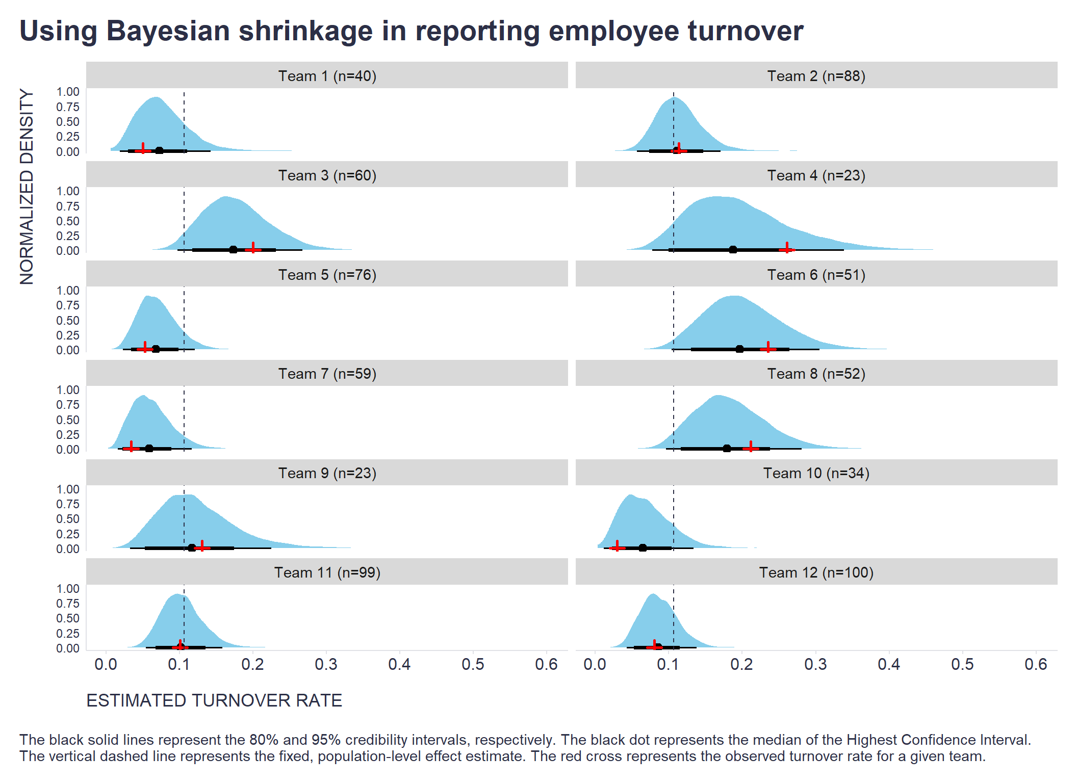
You can see this approach in action on the chart below. The smaller the team and the further its turnover rate is from the company-wide turnover rate (the vertical dashed line), the more the turnover rate estimate for that team is shifted towards the company-wide value (the distance between the red cross and the black dot) - see, for example, teams 4 and 6. For comparison, check teams 12 and 9 that don’t show much of a shrinkage effect due to the big size and small distance from the company-wide turnover rate, respectively.
Show code
# uploading the necessary libraries
library(tidyverse) # data manipulation and dataviz
library(brms) # bayesian stats
library(cmdstanr) # bayesian stats
library(ggdist) # dataviz

# creating artificial data
# setting a seed for reproducibility
set.seed(123)
# number of teams
nTeams <- 12
# generating team sizes ranging from 10 to 100
teamSizes <- sample(10:100, nTeams, replace = TRUE)
# generating 'true' turnover rates from a beta distribution
trueRates <- rbeta(nTeams, 2, 10)
# for each team, simulating the number of employees who left
numberLeft <- rbinom(nTeams, teamSizes, trueRates)
# generating team IDs
teamId <- as.character(1:nTeams)
# creating the data frame
teamsData <- data.frame(teamId, teamSizes, numberLeft)

# fitting multilevel Bayesian logistic regression with wide, uninformative priors
model <- brms::brm(
  numberLeft | trials(teamSizes) ~ 1 + (1 | teamId),
  data = teamsData,
  family = binomial(link = "logit"),
  prior = prior(normal(0, 10), class = "Intercept"),
  chains = 4,
  iter = 5000,
  control = list(adapt_delta = 0.95),
  seed = 123,
  backend = "cmdstanr",
  refresh = 0,
  silent = 2
)

# model summary
#summary(model)
#fixef(model)
#ranef(model)

# extracting the posterior samples
#parnames(model)
posteriorDraws <- as_draws_df(model, variable = "Intercept", regex = TRUE) %>%
  dplyr::select(-.draw, -.chain, -.iteration, -sd_teamId__Intercept) %>%
  tidyr::pivot_longer(cols = -b_Intercept, names_to = "teamId", values_to = "paramValues") %>%
  dplyr::mutate(
    teamId = stringr::str_extract(teamId, "\\d+"),
    team = stringr::str_glue("Team {teamId}"),
    logOdds = paramValues + b_Intercept,
    estimatedTR = exp(logOdds) / (1 + exp(logOdds))
    ) %>%
  dplyr::left_join(teamsData %>% dplyr::select(teamId, teamSizes), by = "teamId") %>%
  dplyr::mutate(
    team = stringr::str_glue("{team} (n={teamSizes})"),
    team = forcats::fct_reorder(factor(team), as.numeric(teamId))
    )

# computing fixed, population-level effect estimate
fixedEffect <- 1 / (1 + exp(-1*fixef(model)[1]))

# computing observed turnover rate by team
observedRT <- teamsData %>%
  dplyr::mutate(team = stringr::str_glue("Team {teamId}")) %>%
  dplyr::mutate(
    observedRT = numberLeft/teamSizes,
    team = stringr::str_glue("{team} (n={teamSizes})"),
    team = forcats::fct_reorder(factor(team), as.numeric(teamId))
  )
Show code
# dataviz
ggplot2::ggplot(data = posteriorDraws, aes(x=estimatedTR, group = team)) +
  ggdist::stat_halfeye(.width = c(0.8, 0.95), point_interval = "median_hdi", fill = "skyblue", normalize = "groups") +
  ggplot2::geom_point(data = observedRT, aes(x = observedRT, y = 0, group = team), color = "red", inherit.aes = F, size = 2.5, shape=3, stroke = 1.5) +
  ggplot2::geom_vline(xintercept = fixedEffect, linetype = "dashed", color = "#2C2F46") +
  ggplot2::facet_wrap(~team, ncol = 2) +
  ggplot2::scale_x_continuous(breaks = seq(0,1,0.1)) +
  ggplot2::labs(
    y = "NORMALIZED DENSITY",
    x = "ESTIMATED TURNOVER RATE",
    title = "Using Bayesian shrinkage in reporting employee turnover",
    caption = "\nThe black solid lines represent the 80% and 95% credibility intervals, respectively. The black dot represents the median of the Highest Confidence Interval.\nThe vertical dashed line represents the fixed, population-level effect estimate. The red cross represents the observed turnover rate for a given team."
  ) +
  ggplot2::theme(
    plot.title = element_text(color = '#2C2F46', face = "bold", size = 21, margin=margin(0,0,12,0)),
    plot.subtitle = element_text(color = '#2C2F46', face = "plain", size = 16, margin=margin(0,0,20,0)),
    plot.caption = element_text(color = '#2C2F46', face = "plain", size = 11, hjust = 0),
    axis.title.x.bottom = element_text(margin = margin(t = 15, r = 0, b = 0, l = 0), color = '#2C2F46', face = "plain", size = 13, hjust = 0),
    axis.title.y.left = element_text(margin = margin(t = 0, r = 15, b = 0, l = 0), color = '#2C2F46', face = "plain", size = 13, hjust = 1),
    axis.text.x = element_text(color = '#2C2F46', face = "plain", size = 12),
    axis.text.y = element_text(color = '#2C2F46', face = "plain", size = 9),
    strip.text.x = element_text(size = 11, face = "plain"),
    axis.line.x = element_line(colour = "#E0E1E6"),
    axis.line.y = element_line(colour = "#E0E1E6"),
    legend.position="",
    panel.background = element_blank(),
    panel.grid.major.y = element_blank(),
    panel.grid.major.x = element_blank(),
    panel.grid.minor = element_blank(),
    axis.ticks.x = element_line(color = "#E0E1E6"),
    axis.ticks.y = element_blank(),
    plot.margin=unit(c(5,5,5,5),"mm"),
    plot.title.position = "plot",
    plot.caption.position =  "plot"
  )
If you are trying to deal with this effect in your reporting practice, can you share the approach you use and serves you well?