Strength-based development and power-law vs. normal distribution of performance

Does a power-law distribution of performance, as opposed to a normal distribution, support the concept of strength-based development?

I just came across the notion that power-law distribution of performance, as opposed to normal distribution, supports the concept of strength-based development. The reasoning was that developing specific strengths can lead to greater success than trying to raise all skills to at least average level.

This was quite surprising to me as my impression was that it was just the opposite. Given the multiplicative nature of power-law distribution, one should - in addition to developing one’s specific strengths - try to avoid having any of the contributing factors at zero or near-zero level, as anything multiplied by zero is still zero. Instead, a normal distribution with its additive nature would support the idea that one can compensate for one’s weaknesses by excessively developing one’s specific strengths.

To validate my impression, I ran a quick and dirty sim of where a person would rank with the same skill profile combining some excessive highs and lows with the middle grounds in a normal and power-law distribution of performance, respectively.

Show code

import pandas as pd
import numpy as np
from scipy.stats import percentileofscore

# creating a dataframe with 7 random variables following a normal distribution
np.random.seed(0)  
data = pd.DataFrame(np.random.normal(0, 1, (10000, 7)), columns=[f'var{i+1}' for i in range(7)])

# transforming these variables to the percentile scale
for col in data.columns:
    data[col] = data[col].rank(pct=True)

# creating two new columns: 'Performance with normal distribution' and 'Performance with power-law distribution'
data['Performance with normal distribution'] = data.sum(axis=1)
data['Performance with power-law distribution'] = data.prod(axis=1)

# creating a skill profile combining some excessive highs and lows with the middle grounds
profile = [1,   0.95,   0.6,    0.4,    0.5,    0.05,   0.025]
profile_normal = sum(profile)
profile_normal_pct = np.round(percentileofscore(data['Performance with normal distribution'], profile_normal), 1)
profile_powerlaw = np.prod(profile)
profile_powerlaw_pct = np.round(percentileofscore(data['Performance with power-law distribution'], profile_powerlaw), 1)

As you can see in the charts attached, the sim seems to support the notion that excessive strengths in the presence of excessive weaknesses help much more under the assumption of normally distributed performance.

Show code

from plotnine import *

# plotting the normal performance distribution
plot = (
  ggplot(data) +
  aes(x='Performance with normal distribution') +
  geom_density(fill = 'grey', color = "white", alpha = 0.7) +
  geom_vline(xintercept = profile_normal, linetype = "dashed") +
  geom_text(
    label=f"A skill profile combining some excessive highs\nand lows with the middle grounds\n(corresponding to {profile_normal_pct} percentile)", 
    x=profile_normal + 0.13, 
    y = 0.45, 
    ha = 'left',
    size = 13
    ) +
  labs(
    title="Performance with normal distribution",
    x = 'Performance',
    y = 'Density'
  ) +
  theme_bw()+
  theme(
    plot_title = element_text(size=20, margin={'b': 12}, ha='left'), 
    axis_title_x = element_text(size=15, margin={'t': 15}), 
    axis_title_y = element_text(size=15, margin={'r': 15}), 
    axis_text_x = element_text(size=10),
    axis_text_y = element_text(size=10),
    panel_grid_major = element_blank(),
    panel_grid_minor = element_blank(),
    figure_size=(13, 6)
  )
)

print(plot)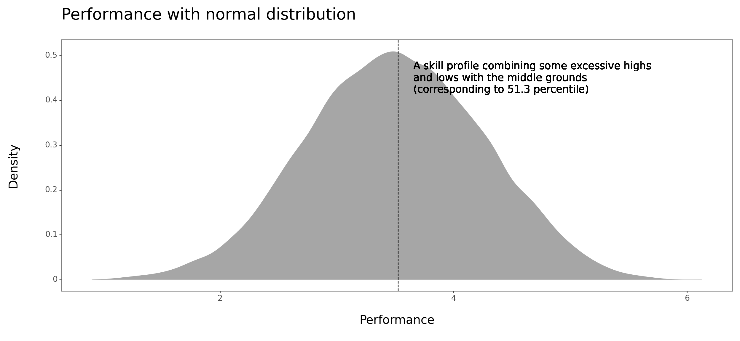

Show code

# plotting the power-law performance distribution
plot = (
  ggplot(data) +
  aes(x='Performance with power-law distribution') +
  geom_density(fill = 'grey', color = "white", alpha = 0.7) +
  geom_vline(xintercept = profile_powerlaw, linetype = "dashed") +
  geom_text(
    label=f"A skill profile combining some excessive highs and lows with the middle grounds\n(corresponding to {profile_powerlaw_pct} percentile)", 
    x=profile_powerlaw + 0.05, 
    y = 50, 
    ha = 'left',
    size = 13
    ) +
  labs(
    title="Performance with power-law distribution",
    x = 'Performance',
    y = 'Density'
  ) +
  theme_bw()+
  theme(
    plot_title = element_text(size=20, margin={'b': 12}, ha='left'), 
    axis_title_x = element_text(size=15, margin={'t': 15}), 
    axis_title_y = element_text(size=15, margin={'r': 15}), 
    axis_text_x = element_text(size=10),
    axis_text_y = element_text(size=10),
    panel_grid_major = element_blank(),
    panel_grid_minor = element_blank(),
    figure_size=(13, 6),
  )
)

print(plot)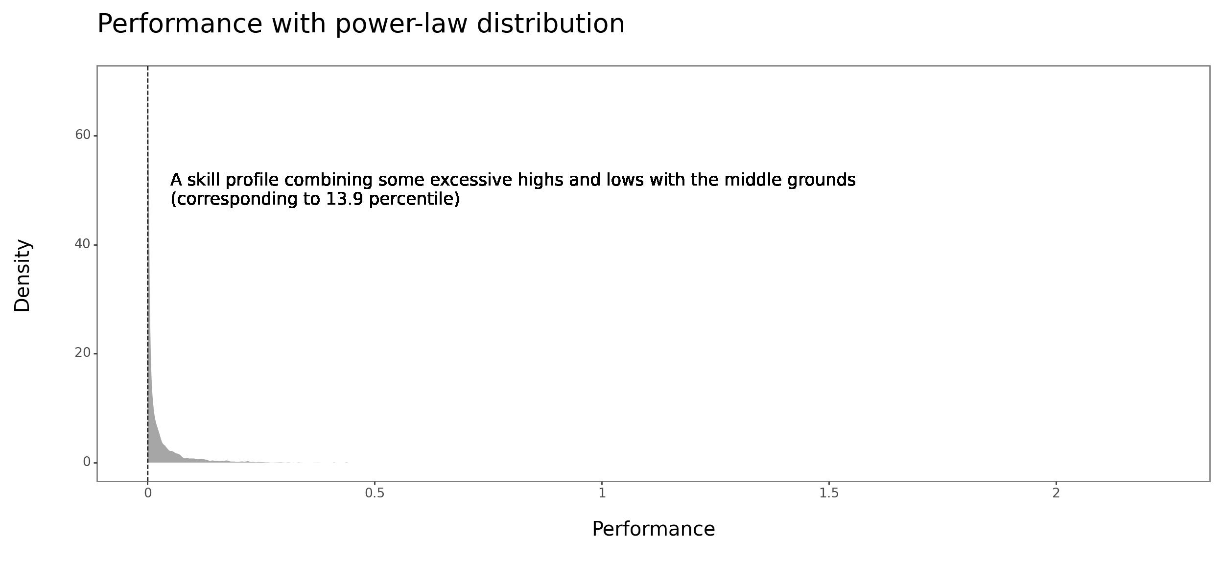

Given these results, one should feel motivated to identify among the mix of factors affecting one’s performance those with multiplicative effect and try to bring them at least to the average level. The question is how one can easily identify which these are. Any tips?